How to Choose a Message Queue? Kafka vs. RabbitMQ

In the last issue, we discussed the benefits of using a message queue. Then we went through the history of message queue products. It seems that nowadays Kafka is the go-to product when we need to use a message queue in a project. However, it’s not always the best choice when we consider specific requirements.

Database-Backed Queue

Let’s use our Starbucks example again. The two most important requirements are:

• Asynchronous processing so the cashier can take the next order without waiting.
• Persistence so customers’ orders are not missed if there is a problem.

Message ordering doesn’t matter much here because the coffee makers often make batches of the same drink. Scalability is not as important either since queues are restricted to each Starbucks location.

The Starbucks queues can be implemented in a database table. The diagram below shows how it works:

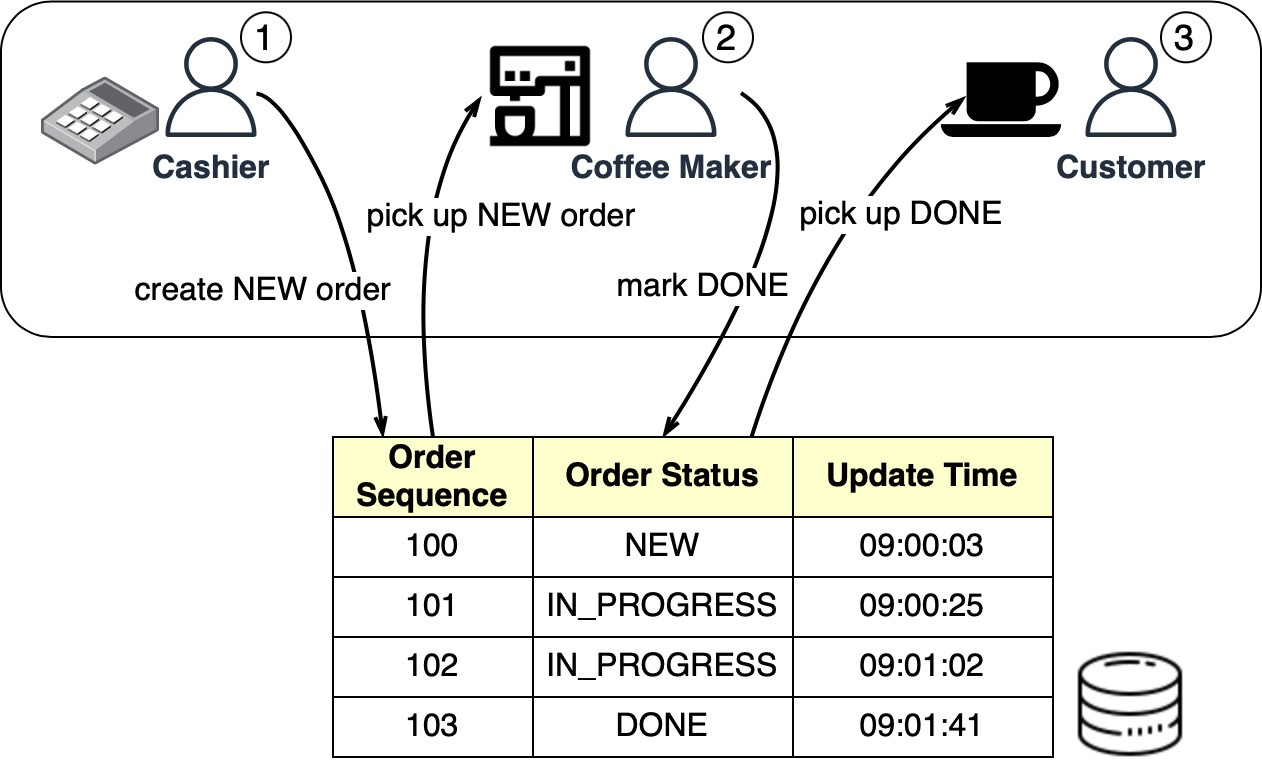
When the cashier takes an order, a new order is created in the database-backed queue. The cashier can then take another order while the coffee maker picks up new orders in batches. Once an order is complete, the coffee maker marks it done in the database. The customer then picks up their coffee at the counter.

A housekeeping job can run at the end of each day to delete complete orders (that is, those with the “DONE status).

For Starbucks’ use case, a simple database queue meets the requirements without needing Kafka. An order table with CRUD (Create-Read-Update-Delete) operations works fine.  

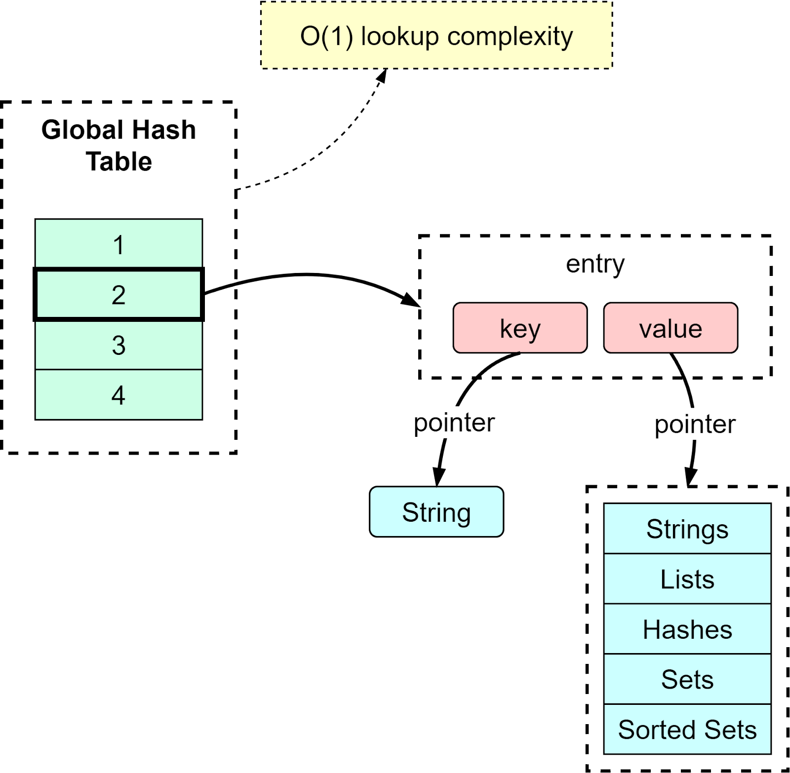
Redis-Backed Queue

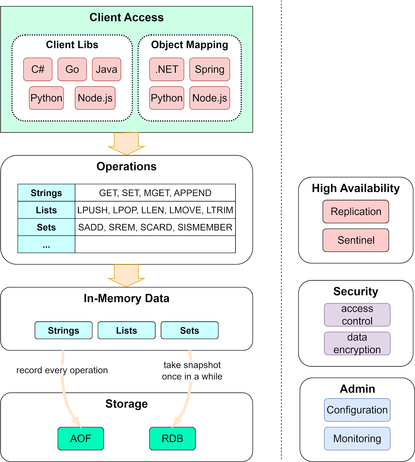
A database-backed message queue still requires development work to create the queue table and read/write from it. For a small startup on a budget that already uses Redis for caching, Redis can also serve as the message queue.

There are 3 ways to use Redis as a message queue:

1. Pub/Sub
2. List
3. Stream

The diagram below shows how they work.

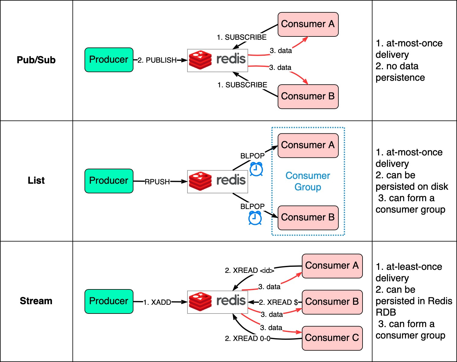
Pub/Sub is convenient but has some delivery restrictions. The consumer subscribes to a key and receives the data when a producer publishes data to the same key. The restriction is that the data is delivered at most once. If a consumer was down and didn’t receive the published data, that data is lost. Also, the data is not persisted on disk. If Redis goes down, all Pub/Sub data is lost. Pub/Sub is suitable for metrics monitoring where some data loss is acceptable.

The List data structure in Redis can construct a FIFO (First-In-First-Out) queue. The consumer uses BLPOP to wait for messages in blocking mode, so a timeout should be applied. Consumers waiting on the same List form a consumer group where each message is consumed by only one consumer. As a Redis data structure, List can be persisted to disk.

Stream solves the restrictions of the above two methods. Consumers choose where to read messages from – “$” for new messages, “<id>” for a specific message id, or “0-0” for reading from the start.

In summary, database-backed and Redis-backed message queues are easy to maintain. If they can’t satisfy our needs, dedicated message queue products are better. We’ll compare two popular options next. 

RabbitMQ vs. Kafka

For large companies that need reliable, scalable, and maintainable systems, evaluate message queue products on the following:

• Functionality
• Performance
• Scalability
• Ecosystem

The diagram below compares two typical message queue products: RabbitMQ and Kafka.

How They Work

RabbitMQ works like a messaging middleware – it pushes messages to consumers then deletes them upon acknowledgment. This avoids message pileups which RabbitMQ sees as problematic.

Kafka was originally built for massive log processing. It retains messages until expiration and lets consumers pull messages at their own pace.

Languages and APIs

RabbitMQ is written in Erlang which makes modifying the core code challenging. However, it offers very rich client API and library support.

Kafka uses Scala and Java but also has client libraries and APIs for popular languages like Python, Ruby, and Node.js.

Performance and Scalability

RabbitMQ handles tens of thousands of messages per second. Even on better hardware, throughput doesn’t go much higher.

Kafka can handle millions of messages per second with high scalability. 

Ecosystem

Many modern big data and streaming applications integrate Kafka by default. This makes it a natural fit for these use cases.

Message Queue Use Cases

Now that we’ve covered the features of different message queues, let’s look at some examples of how to choose the right product.

Log Processing and Analysis

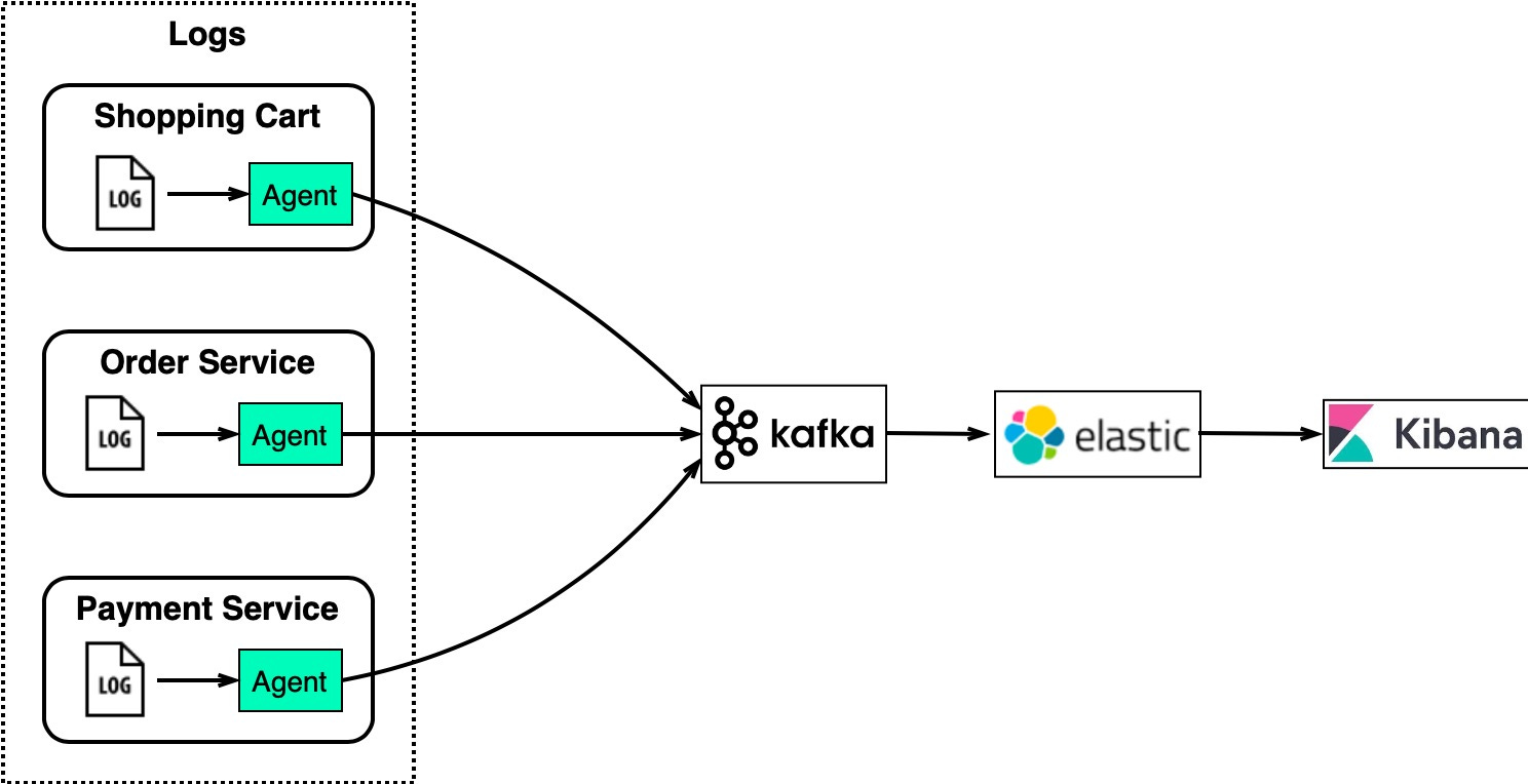
For an eCommerce site with services like shopping cart, orders, and payments, we need to analyze logs to investigate customer orders. 

The diagram below shows a typical architecture uses the “ELK” stack:

• ElasticSearch – indexes logs for full-text search
• LogStash – log collection agent
• Kibana – UI for search and visualizing logs
• Kafka – distributed message queue

Why is Kafka so fast? How does it work?

With data streaming into enterprises at an exponential rate, a robust and high-performing messaging system is crucial. Apache Kafka has emerged as a popular choice for its speed and scalability – but what exactly makes it so fast?

In this issue, we’ll explore:

• Kafka’s architecture and its core components like producer, brokers, and consumers
• How Kafka optimizes data storage and replication
• The optimizations that enable Kafka’s impressive throughput and low latency

Let’s dive into Kafka’s core components first.

Kafka Architecture Distilled

In a typical scenario where Kafka is used as a pub-sub messaging middleware, there are 3 important components: producer, broker, and consumer. The producer is the message sender, and the consumer is the message receiver. The broker is usually deployed in a cluster mode, which handles incoming messages and writes them to the broker partitions, allowing consumers to read from them. 

Note that Kafka is positioned as an event streaming platform, so the term “message”, which is often used in message queues, is not used in Kafka. We call it an “event”. 

The diagram below puts together a detailed view of Kafka’s architecture and client API structure. We can see that although the producer, consumer, and broker are still key to the architecture, it takes more to build a high-throughput, low-latency Kafka. Let’s go through the components one by one.

From a high-level point of view, there are two layers in the architecture: the compute layer and the storage layer.

The Compute Layer

The compute layer, or the processing layer, allows various applications to communicate with Kafka brokers via APIs. 

The producers use the producer API. If external systems like databases want to talk to Kafka, it also provides Kafka Connect as integration APIs.

The consumers talk to the broker via consumer API. In order to route events to other data sinks, like a search engine or database, we can use Kafka Connect API. Additionally, consumers can perform streaming processing with Kafka Streams API. If we deal with an unbounded stream of records, we can create a KStream. The code snippet below creates a KStream for the topic “orders” with Serdes (Serializers and Deserializers) for key and value. If we just need the latest status from a changelog, we can create a KTable to maintain the status. Kafka Streams allows us to perform aggregation, filtering, grouping, and joining on event streams. 

final KStreamBuilder builder = new KStreamBuilder();final KStream<String, OrderEvent> orderEvents = builder.stream(Serdes.String(), orderEventSerde, "orders");

While Kafka Streams API works fine for Java applications, sometimes we might want to deploy a pure streaming processing job without embedding it into an application. Then we can use ksqlDB, a database cluster optimized for stream processing. It also provides a REST API for us to query the results.

We can see that with various API support in the compute layer, it is quite flexible to chain the operations we want to perform on event streams. For example, we can subscribe to topic “orders”, aggregate the orders based on products, and send the order counts back to Kafka in the topic “ordersByProduct”, which another analytics application can subscribe to and display. 

The Storage Layer

This layer is composed of Kafka brokers. Kafka brokers run on a cluster of servers. The data is stored in partitions within different topics. A topic is like a database table, and the partitions in a topic can be distributed across the cluster nodes. Within a partition, events are strictly ordered by their offsets. An offset represents the position of an event within a partition and increases monotonically. The events persisted on brokers are immutable and append-only, even deletion is modeled as a deletion event. So, producers only handle sequential writes, and consumers only read sequentially.

A Kafka broker’s responsibilities include managing partitions, handling reads and writes, and managing replications of partitions. It is designed to be simple and hence easy to scale. We will review the broker architecture in more detail.

Since Kafka brokers are deployed in a cluster mode, there are two necessary components to manage the nodes: the control plan and the data plane.

Control Plane

The control plane manages the metadata of the Kafka cluster. It used to be Zookeeper that managed the controllers: one broker was picked as the controller. Now Kafka uses a new module called KRaft to implement the control plane. A few brokers are selected to be the controllers. 

Why was Zookeeper eliminated from the cluster dependency? With Zookeeper, we need to maintain two separate types of systems: one is Zookeeper, and the other is Kafka. With KRaft, we just need to maintain one type of system, which makes the configuration and deployment much easier than before. Additionally, KRaft is more efficient in propagating metadata to brokers.

We won’t discuss the details of the KRaft consensus here. One thing to remember is the metadata caches in the controllers and brokers are synchronized via a special topic in Kafka.

Data Plane

The data plane handles the data replication. The diagram below shows an example. Partition 0 in the topic “orders” has 3 replicas on the 3 brokers. The partition on Broker 1 is the leader, where the current data offset is at 4; the partitions on Broker 2 and 3 are the followers where the offsets are at 2 and 3. 

Step 1 – In order to catch up with the leader, Follower 1 issues a FetchRequest with offset 2, and Follower 2 issues a FetchRequest with offset 3. 

Step 2 – The leader then sends the data to the two followers accordingly.

Step 3 – Since followers’ requests implicitly confirm the receipts of previously fetched records, the leader then commits the records before offset 2.

Record

Kafka uses the Record class as an abstraction of an event. The unbounded event stream is composed of many Records. 

There are 4 parts in a Record：

1. Timestamp
2. Key
3. Value
4. Headers (optional)

The key is used for enforcing ordering, colocating the data that has the same key, and data retention. The key and value are byte arrays that can be encoded and decoded using serializers and deserializers (serdes). 

Broker

We discussed brokers as the storage layer. The data is organized in topics and stored as partitions on the brokers. Now let’s look at how a broker works in detail.

Step 1: The producer sends a request to the broker, which lands in the broker’s socket receive buffer first. 

Steps 2 and 3: One of the network threads picks up the request from the socket receive buffer and puts it into the shared request queue. The thread is bound to the particular producer client.

Step 4: Kafka’s I/O thread pool picks up the request from the request queue.

Steps 5 and 6: The I/O thread validates the CRC of the data and appends it to a commit log. The commit log is organized on disk in segments. There are two parts in each segment: the actual data and the index.

Step 7: The producer requests are stashed into a purgatory structure for replication, so the I/O thread can be freed up to pick up the next request.

Step 8: Once a request is replicated, it is removed from the purgatory.  A response is generated and put into the response queue. 

Steps 9 and 10: The network thread picks up the response from the response queue and sends it to the corresponding socket send buffer. Note that the network thread is bound to a certain client. Only after the response for a request is sent out, will the network thread take another request from the particular client.

A Crash Course in Redis

Redis (Remote Dictionary Server) is an open-source (BSD licensed), in-memory database, often used as a cache, message broker, or streaming engine. It has rich support for data structures, including basic data structures like String, List, Set, Hash, SortedSet, and probabilistic data structures like Bloom Filter, and HyperLogLog. 

Redis is super fast. We can run Redis benchmarks with its own tool. The throughput can reach nearly 100k requests per second.

In this issue, we will discuss why Redis is fast in its architectural design.

---

Redis Architecture

Redis is an in-memory key-value store. There are several important functions：

1. The data structures used for the values
2. The operations allowed on the data structures
3. Data persistence
4. High availability

Below is a high-level diagram of Redis’ architecture. Let’s walk through them one by one.

Client Libraries

There are two types of clients to access Redis: one supports connections to the Redis database, and the other builds on top of the former and supports object mappings.

Redis supports a wide range of languages, allowing it to be used in a variety of applications. In addition, the OM client libraries allow us to model, index, and query documents.

Data Operations

Redis has rich support for value data types, including Strings, Lists, Sets, Hashes, etc. As a result, Redis is suitable for a wide range of business scenarios. Depending on the data types, Redis supports different operations. 

The basic operations are similar to a relational database, which supports CRUD (Create-Read-Update-Delete):

• GET: Retrieve the value of a key
• PUT: Create a new key-value pair or update an existing key
• DELETE: Delete a key-value pair 

The data structures and operations are an important reason why Redis is so efficient. We will cover more in later sections.

In-Memory v.s. On-Disk

Redis holds the data in memory. The data reads and writes in memory are generally 1,000X – 10,000X faster than disk reads/writes. See the below diagram for details. 

However, if the server is down, all the data will be lost. So Redis designs on-disk persistence as well for fast recovery.

Redis has 4 options for persistence:

1. AOF (Append Only File).

AOF works like a commit log, recording each write operation to Redis. So when the server is restarted, the write operations can be replayed and the dataset can be reconstructed.

2. RDB (Redis Database).

RDB performs point-in-time snapshots at a predefined interval.

3. AOF and RDB.

This persistence method combines the advantages of both AOF and RDB, which we will cover later.

4. No persistence.

Persistence can be entirely disabled in Redis. This is sometimes used when Redis is a cache for smaller datasets, 

Clustering

Redis uses a leader-follower replication to achieve high availability. We can configure multiple replicas for reads to handle concurrent read requests. These replicas automatically connect to the master after restarts and hold an exact copy of the leader instance.

When the Redis cluster is not used, Redis Sentinel provides high availability including failover, monitoring, and configuration management.

Security and Administration

Redis is often used as a cache and can hold sensitive data, so it is designed to be accessed via trusted clients inside trusted environments. Redis security module is responsible for managing the access control layer and authorizing the valid operations to be performed on the data.

Redis also provides an admin interface for configuring and managing the cluster. Persistence, replication, and security configurations can all be done via the admin interface.

Now we have covered the basic components of Redis architecture, we will dive into the design details that make Redis fast.

In-Memory Data Structures

Redis is not the only in-memory database product in the market. But how can it achieve microsecond-level data access latency and become a popular choice for many companies?

One important reason is that storing data in memory allows for more flexible data structures. These data structures don’t need to go through the process of serialization and deserialization like normal on-disk data structures do, so can be optimized for fast reads and writes.

Key-Value Mappings

Redis uses a hash table to hold all key-value pairs. The elements in the hash table hold the pointers to a key-value pair entry. The diagram below illustrates how the global hash table is structured. 

With the hash table, we can look up key-value pairs with O(1) time complexity. 

Like all hash tables, when the number of keys keeps growing, there can be hash conflicts, which means different keys fall into the same hash bucket. Redis solves this by chaining the elements in the same hash bucket. When the chains become too long, Redis will perform a rehash by leveraging two global hash tables.  

Value Types

The diagram below shows how Redis implements the common data structures. String type has only one implementation, the SDS (Simple Dynamic Strings). List, Hash, Set, and SortedSet all have two types of implementations.

Note that Redis 7.0 changed List implementation to quicklist, and ZipList was replaced by listpack.

Besides these 5 basic data structures, Redis later added more data structures to support more scenarios. The diagram below lists the operations allowed on basic data structures and the usage scenarios.

These data types cover most of the usage of a website. For example, geospatial data stores coordinates that can be used by a ride-hailing application like Uber; HyperLogLog calculates cardinality for massive amounts of data, suitable for counting unique visitors for a large website; Stream is used for message queues and can compensate the problems with List.

Now let’s look at why these underlying implementations are efficient.

SDS

Redis SDS stores sequences of bytes. It operates the data stored in buf array in a binary way, so SDS can store not only text but also binary data like audio, video, and images.

The string length operation on an SDS has a time complexity of O(1) because the length is recorded in len attribute. The space is pre-allocated for an SDS, with free attribute recording the free space for future usage. The SDS API is thus safe, and there is no risk of overflow.

The diagram below shows the attributes of an SDS.

Zip List

A zip list is similar to an array. Each element of the array holds one piece of data. However, unlike an array, a zip list has 3 fields in the header: 

• zlbytes – the length of the list
• zltail – the offset at the end of the list
• zllen – the number of entries in the list

The zip list also has a zlend at the end, which indicates the end of the list.

In a zip list, locating the first or the last element is O(1) time complexity because we can directly find them by the fields in the header. Locating other elements needs to go through the elements one by one, and the time complexity is O(N).

Topics and References for Az-303 Exam

Technical Reference

Difference between authentication protocols: https://www.getkisi.com/blog/authentication-protocols-overview

Study guide for Azure Az-303 certification: https://www.thomasmaurer.ch/2020/03/az-303-study-guide-azure-architect-technologies/

Implement and Monitor an Azure Infrastructure (50-55%)

Implement cloud infrastructure monitoring

• monitor security
  • Strengthen your security posture with Azure Security Center
  • Security Control: Logging and Monitoring
  • Azure infrastructure monitoring
• monitor performance
  • Create diagnostic setting to collect platform logs and metrics in Azure
  • Create diagnostic setting in Azure using a Resource Manager template
  • Metric Baseline – Get
  • Azure Monitor overview
  • Quickstart: Monitor an Azure resource with Azure Monitor
  • Azure Monitor Workbooks
  • Azure Monitor workbook visualizations
  • Collect data from an Azure virtual machine with Azure Monitor
• monitor health and availability
  • Azure Service Health
  • Resource Health overview
• monitor cost
  • Monitoring your cloud costs
  • Use cost alerts to monitor usage and spending
  • Download or view your Azure billing invoice and daily usage data
• configure advanced logging
  • What is Application Insights?
  • Overview of Insights in Azure Monitor
• configure logging for workloads
  • Logs in Azure Monitor
• initiate automated responses by using Action Groups
  • Create and manage action groups in the Azure portal
• configure and manage advanced alerts
  • Create, view, and manage log alerts using Azure Monitor
  • Manage alert instances with unified alerts
  • Create diagnostic setting to collect platform logs and metrics in Azure
  • Overview of alerts in Microsoft Azure
  • Create a Log Analytics workspace in the Azure portal

Implement storage accounts

• select storage account options based on a use case
  • Storage account overview
  • Introduction to Azure Storage
• configure Azure Files and blob storage
  • Introduction to Azure Blob storage
  • Create an Azure file share
• configure network access to the storage account
  • Configure Azure Storage firewalls and virtual networks
• implement Shared Access Signatures and access policies
  • Delegate access with a shared access signature
  • Grant limited access to Azure Storage resources using shared access signatures (SAS)
• implement Azure AD authentication for storage
  • Authorize access to blobs and queues using Azure Active Directory
• manage access keys
  • Manage storage account access keys
• implement Azure storage replication
  • Azure Storage redundancy
  • Disaster recovery and account failover (preview)
• implement Azure storage account failover
  • Initiate a storage account failover (preview)

Implement VMs for Windows and Linux

• configure High Availability
  • Availability options for virtual machines in Azure
  • Manage the availability of Windows virtual machines in Azure
• configure storage for VMs
  • Attach a managed data disk to a Windows VM by using the Azure portal
  • Attach a data disk to a Windows VM with PowerShell
  • What disk types are available in Azure?
• select virtual machine size
  • Sizes for Windows virtual machines in Azure
  • Sizes for Linux virtual machines in Azure
• implement Azure Dedicated Hosts
  • Deploy VMs to dedicated hosts using the portal
  • Azure Dedicated Hosts
• deploy and configure scale sets
  • What are virtual machine scale sets?
• configure Azure Disk Encryption
  • Azure Disk Encryption for Linux VMs
  • Azure Disk Encryption for Windows VMs

Automate deployment and configuration of resources

• save a deployment as an Azure Resource Manager template
  • Download the template for a VM
• modify Azure Resource Manager template
  • Extend Azure Resource Manager template functionality
  • Azure Resource Manager templates overview
  • Tutorial: Create and deploy your first Azure Resource Manager template
• evaluate location of new resources
  • Conditional deployment in Resource Manager templates
  • Set resource location in Resource Manager template
• configure a virtual disk template
  • Create a VM from a VHD by using the Azure portal
• deploy from a template
  • Download the template for a VM
• manage a template library
  • Azure Resource Manager templates overview
• create and execute an automation runbook
  • Start a runbook in Azure Automation

Implement virtual networking

• implement VNet to VNet connections
  • Configure a VNet-to-VNet VPN gateway connection by using the Azure portal
• implement VNet peering
  • Virtual network peering
  • Create, change, or delete a virtual network peering

Implement Azure Active Directory

• add custom domains
  • Add your custom domain name using the Azure Active Directory portal
• configure Azure AD Identity Protection
  • What is Azure Active Directory Identity Protection?
• implement self-service password reset
  • Plan an Azure Active Directory self-service password reset
  • How it works: Azure AD self-service password reset
  • Licensing requirements for Azure AD self-service password reset
• implement Conditional Access including MFA
  • Conditional Access: Require MFA for all users
  • Conditional Access: Risk-based Conditional Access
• configure user accounts for MFA
  • Tutorial: Secure user sign-in events with Azure Multi-Factor Authentication
• configure fraud alerts
  • Reports in Azure Multi-Factor Authentication
  • Configure Azure Multi-Factor Authentication settings
• configure bypass options
  • Configure Azure Multi-Factor Authentication settings
• configure Trusted IPs
  • Quickstart: Configure named locations in Azure Active Directory
  • What is the location condition in Azure Active Directory Conditional Access?
• configure verification methods
  • Change your two-factor verification method and settings
  • What is the Additional verification page?
• implement and manage guest accounts
  • What is guest user access in Azure Active Directory B2B?
  • Manage guest access with Azure AD access reviews
  • Quickstart: Add guest users to your directory in the Azure portal
• manage multiple directories
  • Understand how multiple Azure Active Directory tenants interact

Implement and manage hybrid identities

• install and configure Azure AD Connect
  • Custom installation of Azure AD Connect
  • Select which installation type to use for Azure AD Connect
• identity synchronization options
  • Azure AD Connect sync: Understand and customize synchronization
  • Azure Active Directory Hybrid Identity Design Considerations
• configure and manage password sync and password writeback
  • Implement password hash synchronization with Azure AD Connect sync
  • Tutorial: Enable Azure Active Directory self-service password reset writeback to an on-premises environment
  • Azure AD Connect: Enabling device writeback
  • What is password writeback?
• configure single sign-on
  • Azure Active Directory Seamless Single Sign-On: Quick start
  • Azure Active Directory Seamless Single Sign-On: Frequently asked questions
• use Azure AD Connect Health
  • Azure Active Directory Connect Health operations
  • What is Azure AD Connect?

Implement Management and Security Solutions (25-30%)

Manage workloads in Azure

• migrate workloads using Azure Migrate
  • About Azure Migrate
  • Prepare VMware VMs for assessment and migration to Azure
  • Assess VMware VMs by using Azure Migrate Server Assessment
  • Select a VMware migration option
  • Migrate VMware VMs to Azure (agentless)
  • Migrate VMware VMs to Azure (agent-based)
• implement Azure Backup for VMs
  • An overview of Azure VM backup
  • Get improved backup and restore performance with Azure Backup Instant Restore capability
• implement disaster recovery
  • Set up disaster recovery to a secondary Azure region for an Azure VM
• implement Azure Update Management
  • Update Management solution in Azure
  • Enable Update Management, Change Tracking, and Inventory solutions on multiple VMs
  • Manage updates and patches for your Azure VMs

Implement load balancing and network security

• implement Azure Load Balancer
  • Tutorial: Balance internal traffic load with a Basic load balancer in the Azure portal
  • Create an internal load balancer by using the Azure PowerShell module
  • Quickstart: Create a Load Balancer to load balance VMs using the Azure portal
• implement an application gateway
  • Application Gateway configuration overview
• implement a Web Application Firewall
  • Azure Web Application Firewall on Azure Application Gateway
• implement Azure Firewall
  • Tutorial: Deploy and configure Azure Firewall using the Azure portal
• implement the Azure Front Door Service
  • What is Azure Front Door Service?
  • Quickstart: Create a Front Door for a highly available global web application
• implement Azure Traffic Manager
  • What is Traffic Manager?
  • Quickstart: Create a Traffic Manager profile using the Azure portal
• implement Network Security Groups and Application Security Groups
  • Security groups
  • Create, change, or delete a network security group
• implement Bastion
  • Create an Azure Bastion host

Implement and manage Azure governance solutions

• create and manage hierarchical structure that contains management groups, subscriptions and resource groups
  • Azure Resource Manager overview
  • Organize your resources with Azure management groups
  • Create management groups for resource organization and management
  • Manage Azure Resource Manager resource groups by using the Azure portal
  • Azure subscription and service limits, quotas, and constraints
• assign RBAC roles
  • Add or remove role assignments using Azure RBAC and the Azure portal
• create a custom RBAC role
  • Custom roles for Azure resources
  • Tutorial: Create a custom role for Azure resources using Azure PowerShell
• configure access to Azure resources by assigning roles
  • Tutorial: Grant a user access to Azure resources using RBAC and the Azure portal
• configure management access to Azure
  • Manage access to Azure management with Conditional Access
  • Manage access to Azure resources with Azure AD Privileged Identity Management
  • Add or remove role assignments using Azure RBAC and the Azure portal
• interpret effective permissions
  • What is role-based access control (RBAC) for Azure resources?
  • Quickstart: View the access a user has to Azure resources
• set up and perform an access review
  • What are Azure AD access reviews?
• implement and configure an Azure Policy
  • What is Azure Policy?
  • Quickstart: Create a policy assignment to identify non-compliant resources
  • Tutorial: Create and manage policies to enforce compliance
• implement and configure an Azure Blueprint
  • What is Azure Blueprints?
  • Quickstart: Define and assign a blueprint in the portal

Manage security for applications

• implement and configure KeyVault
  • What is Azure Key Vault?
  • About keys, secrets, and certificates
• implement and configure Azure AD Managed Identities
  • What are managed identities for Azure resources?
  • Use a Windows VM system-assigned managed identity to access Resource Manager
• register and manage applications in Azure AD
  • Tutorial: Register an application in Azure Active Directory B2C

Implement Solutions for Apps (10-15%)

Implement an application infrastructure

• create and configure Azure App Service
  • App Service overview
  • Introduction to the App Service Environments
  • Custom configuration and application settings in Azure Web Sites
  • Configure an App Service app in the Azure portal
  • Buy a custom domain name for Azure App Service
  • Create an ASP.NET Core web app in Azure
• create an App Service Web App for Containers
  • Deploy a custom Linux container to Azure App Service
• create and configure an App Service plan
  • Azure App Service plan overview
  • Manage an App Service plan in Azure
• configure an App Service
  • Custom configuration and application settings in Azure Web Sites
  • Configure an App Service app in the Azure portal
  • Buy a custom domain name for Azure App Service
• configure networking for an App Service
  • Networking considerations for an App Service Environment
  • App Service networking features
  • Integrate your app with an Azure Virtual Network
• create and manage deployment slots
  • Set up staging environments in Azure App Service
• implement Logic Apps
  • Overview – What is Azure Logic Apps?
  • Quickstart: Create your first workflow by using Azure Logic Apps – Azure portal
  • Quickstart: Create automated tasks, processes, and workflows with Azure Logic Apps – Visual Studio
  • Quickstart: Create and manage logic app workflow definitions by using Visual Studio Code
• implement Azure Functions
  • An introduction to Azure Functions
  • Azure Functions triggers and bindings concepts
  • Azure Functions trigger and binding example
  • Azure Functions triggers and bindings concepts
  • Azure Functions trigger and binding example
  • Azure Functions HTTP triggers and bindings overview
  • What are Durable Functions?

Implement container-based applications

• create a container image
  • Tutorial: Build and deploy container images in the cloud with Azure Container Registry Tasks
  • Tutorial: Create container images on a Linux Service Fabric cluster
  • Tutorial: Create a container image for deployment to Azure Container Instances
• configure Azure Kubernetes Service
  • Azure Kubernetes Service (AKS)
  • Quickstart: Deploy an Azure Kubernetes Service (AKS) cluster using the Azure portal
• publish and automate image deployment to the Azure Container Registry
  • Push your first image to a private Docker container registry using the Docker CLI
  • Tutorial: Build and deploy container images in the cloud with Azure Container Registry Tasks
• publish a solution on an Azure Container Instance
  • What is Azure Container Instances?
  • Quickstart: Deploy a container instance in Azure using the Azure portal
  • Quickstart: Deploy a container instance in Azure using the Azure CLI

Implement and Manage Data Platforms (10-15%)

Implement NoSQL databases

• configure storage account tables
  • Azure Table storage overview
  • Understanding the Table service data model
• select appropriate CosmosDB APIs
  • Choose the appropriate API for Azure Cosmos DB storage (Microsoft Learn module)
  • Welcome to Azure Cosmos DB
• set up replicas in CosmosDB
  • Choose the right consistency level
  • Consistency levels and Azure Cosmos DB APIs
  • Consistency, availability, and performance tradeoffs

Implement Azure SQL databases

• configure Azure SQL database settings
  • What is the Azure SQL Database service? 
  • Quickstart: Create a single database in Azure SQL Database using the Azure portal, PowerShell, and Azure CLI
  • Choose the right deployment option in Azure SQL
• implement Azure SQL Database managed instances
  • SQL managed instance
  • What is Azure SQL Database managed instance?
  • Quickstart: Create an Azure SQL Database managed instance
• configure HA for an Azure SQL database
  • High-availability and Azure SQL Database
• publish an Azure SQL database
  • Azure SQL database deployment
  • Tutorial: Deploy your ASP.NET app and Azure SQL Database code by using Azure DevOps Projects

Using Git

What is Git ?

Git is a open source version control system for tracking changes and coordinating work on files. It is primarily used for source code management in software development, but it can be used to keep track of changes in any set of files. As a distributed revision control system it is aimed at speed, data integrity, and support for distributed, non-linear workflows.

Git was created by Linus Torvalds in 2005 for development of the Linux kernel, with other kernel developers contributing to its initial development.

As with most other distributed version control systems, and unlike most client–server systems, every Git directory on every computer is a full-fledged repository with complete history and full version tracking abilities, independent of network access or a central server.

Scenarios:

• Add existing project to remote git repository using command line.

Follow below steps if you want to add existing project/solution to remote git repository

1. Lets first add existing solution to local git repository. Go to the folder with your solution/work-space on local machine.
2. Add .gitignore file to the project folder. You can search for gitignore template online for different type of projects e.g.: Visual Studio.
3. Open command prompt and change directory to your project path.
4. Create a new local git repository using command :  git init
5. This is optional step but useful sometimes. Perform a dry run to check if all expected files will be added to the local repository using command: git add –all –dry-run 
6. Add and commit files to the repository using(Add and commit can be done separately) : git add –all && git commit -m “<Comments text>”.                                    [ You now have everything setup in your git repository. Time to create remote repository ]
7. Create a folder to house new git repository in the remote location.
8. Create a bare/blank git repository in the remote directory using: git init –bare
9. Go back to your local project repository.
10. Link remote repository: git remote add origin <remote repo directory>
11. Push the code/changes to remote repository using: git push origin -all

 

 

The Journey Begins

Thanks for joining me!

Good company in a journey makes the way seem shorter. — Izaak Walton